Design of Experiments
- Feb 1, 2025
- 11 min read
Updated: Feb 26, 2025
Hey everyone! Welcome back to my blog :D. Hope you're all doing great!
In this blog, I'll be tackling a case study using the Design of Experiments (DOE) method. I'll walk you guys through how I used both full and fractional analyses, including graphs, tables and key points along the way! As always, I'll wrap up with a reflection summarising my experiences solving this case study :))
Alright! Without further ado, let's dive right in! But wait - before we jump into the fancy MS Excel stuff, let me give you guys a brief background on what the DOE method is all about.
The DOE method is a statistics-based approach to designing experiments. It helps us figure out the significance of different factors in an experiment and how they interact, all while being as efficient as possible! In simple terms, it’s about strategically choosing the minimum number of runs needed to analyse all the factors - perfect for us lazy folks.
OKAY, let's actually start now!
This case study is all about figuring out what affects the yield of microwave popcorn! We’ll be looking at three key factors: the size of the bowl, how long it’s microwaved, and the microwave power setting. By the end, we’ll uncover what’s causing those annoying unpopped kernels, because biting into those things SUCKS :(
We will start off by carrying out the full factorial method, where we will analyse all 8 runs to figure out the significance and interactions between the factors. Yes, this is the tedious, tiring, and inefficient way of doing it - but we need to use this method first to later prove that the fractional factorial method is more efficient (subtle foreshadowing). If not, I can't prove that what I learn in school is useful :(
Oh yeah, my admin no. ends with 16. So yeah, I'll be replacing XX with 16 accordingly. I'll also be referring to the diameter, microwaving time and power as Factor A, B and C respectively for convenience :D.
Here's the data for the 8 runs that I will be using for the full factorial method:
Run Order | A | B | C | Bullets (grams) |
1 | + | - | - | 3.16 |
2 | - | + | - | 2.16 |
3 | - | - | + | 0.74 |
4 | + | + | - | 1.16 |
5 | + | - | + | 0.95 |
6 | + | + | + | 0.32 |
7 | - | + | + | 0.16 |
8 | - | - | - | 3.12 |
First, let's examine the significance of each factor.
To do so, I first need to find the average weight of the bullets for the when the high levels and low levels of each factor are used respectively.
Okay that sounds really stupid. I'll just provide an example to make it easier for you guys :DD
So, the runs where a high level of Factor A is used are runs 1, 4, 5 and 6. The weight of the bullets for these runs are 3.16g, 1.16g, 0.95g and 0.32g respectively.
I'll then need to find out the average weight for these 4 runs. Which is:
(3.16 + 1.16 + 0.95 + 0.32)/4 = 1.3975g
After that, I’ll do the same thing for the low level of A and repeat the process for all the other factors! Don’t worry, I’m not going to bore you guys by walking through the calculations for each factor LOL. Instead, I’ll just show all my calculations below, which I've done in MS Excel.
Factor A | |||||||||||||
Runs where A is +: | 3.16 | + | 1.16 | + | 0.95 | + | 0.32 | = | 5.59 | Average = | 1.3975 | ||
Runs where A is -: | 2.16 | + | 0.74 | + | 0.16 | + | 3.12 | = | 6.18 | Average = | 1.545 | ||
Difference = | -0.1475 | ||||||||||||
Factor B | |||||||||||||
Runs where B is +: | 2.16 | + | 1.16 | + | 0.32 | + | 0.16 | = | 3.8 | Average = | 0.95 | ||
Runs where B is -: | 3.16 | + | 0.74 | + | 0.95 | + | 3.12 | = | 7.97 | Average = | 1.9925 | ||
Difference = | -1.0425 | ||||||||||||
Factor C | |||||||||||||
Runs where C is +: | 0.74 | + | 0.95 | + | 0.32 | + | 0.16 | = | 2.17 | Average = | 0.5425 | ||
Runs where C is -: | 3.16 | + | 2.16 | + | 1.16 | + | 3.12 | = | 9.6 | Average = | 2.4 | ||
Difference = | -1.8575 |
(that's actually so cool like when you copy from excel and paste onto wix it's a table that can move like WHY CANT WORD DO THAT)
Alright! With the calculations out of the way, I can now plot a graph that helps me compare and rank the significance of each factor!

Based on this plot, the ranking from most significant to least significant is Factor C (Power), Factor B (Microwaving time), Factor A (Diameter). This is because the steeper the plot, the greater the significance of the factor. Since the ranking for steepness of the plot from steepest to gentlest is Factor C, Factor B, Factor A, the ranking for the significance of each factor from most to least significant is also Factor C, Factor B, Factor A.
With the analysis of the significance of each factor out of the way, we can now move on to studying the interactions between them!
To perform this analysis, I'll need to calculate a set of values. I don't think I can explain exactly what I'm calculating in words, so, I will present all my calculations on a table again, which should be easy to understand :)
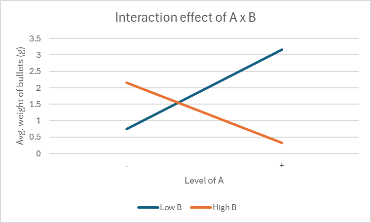
Let's first analyse the significance of the interaction between Factor A and B!
At Low B | |||||||||
Runs where A is +: | 3.16 | + | 0.95 | = | 4.11 | Average = | 2.055 | ||
Runs where A is -: | 0.74 | + | 3.12 | = | 3.86 | Average = | 1.93 | ||
Difference = | 0.125 | ||||||||
At High B | |||||||||
Runs where A is +: | 1.16 | + | 0.32 | = | 1.48 | Average = | 0.74 | ||
Runs where A is -: | 2.16 | + | 0.16 | = | 2.32 | Average = | 1.16 | ||
Difference = | -0.42 |
Okay, maybe I should try to explain this LOL
Basically, what I've done above is calculate the average values for when:
High A and Low B are used
High A and High B are used
Low A and Low B are used
Low A and High B are used
So yeah, I'll repeat this when analysing the interactions between other factors, but let's focus on these two first. With the values I've obtained from the table found above, I can now plot a graph!

From this graph, we can see that the gradients of both lines are different, since the line for Low B has a positive gradient, while the line for High B has a negative gradient. We can hence conclude that there is a significant interaction between Factor A and B. YAY! Now, let's do the same thing two more times to analyse the interactions between the rest of the factors.
Here are the calculations for A x C:
At Low C | |||||||||
Runs where A is +: | 3.16 | + | 1.16 | = | 4.32 | Average = | 2.16 | ||
Runs where A is -: | 2.16 | + | 3.12 | = | 5.28 | Average = | 2.64 | ||
Difference = | -0.48 | ||||||||
At High C | |||||||||
Runs where A is +: | 0.95 | + | 0.32 | = | 1.27 | Average = | 0.635 | ||
Runs where A is -: | 0.74 | + | 0.16 | = | 0.9 | Average = | 0.45 | ||
Difference = | 0.185 |
And here's the graph!

This graph is very similar to the A x B one! We can see that the gradients of both lines are different, since the line for Low C has a negative gradient, while the line for High B has a positive gradient. So, the interactions between A and C can be considered significant!
Alright, we have one more graph to plot, and we're done with the full factorial method!
These are the calculations for B x C:
At Low C | |||||||||
Runs where B is +: | 2.16 | + | 1.16 | = | 3.32 | Average = | 1.66 | ||
Runs where B is -: | 3.16 | + | 3.12 | = | 6.28 | Average = | 3.14 | ||
Difference = | -1.48 | ||||||||
At High C | |||||||||
Runs where B is +: | 0.32 | + | 0.16 | = | 0.48 | Average = | 0.24 | ||
Runs where B is -: | 0.74 | + | 0.95 | = | 1.69 | Average = | 0.845 | ||
Difference = | -0.605 |
And here's the last graph for full factorial!

This graph's a bit different compared to the last two. In this graph, the lines are ALMOST parallel, showing that the gradients of both lines only differ by a bit. This means that there is only a small interaction between Factor B and C (NOT SIGNIFICANT).
OKAY! We've finally finished the full factorial method! Before we move on to the fractional factorial method. Let's conclude what we've found.
Through this analysis, we've identified that Factor C is the most significant factor, while Factor A is the least. We've also observed significant interactions between all factors, except between B and C!
It's now time to carry out the fractional factorial method!
This method will involve the exact same steps as the full factorial method. However, this time, we will strategically select only 4 runs to analyse to make things easier for us!
Let's first go through the thought process behind picking the runs to analyse :D
We need to pick 4 runs that ensure statistical orthogonality. Wow, big words. Well, to put it in layman terms, we need to pick four runs where all factors occur (both high and low levels), the same number of times.
Now, how exactly do I do that?

Pardon the quality, I had to take a screenshot of a slide from class and crop it. This is the combination of runs we've always been advised to use in class, so it's been my go-to method, and I'm probably sticking with this forever HAHAHA.
Through comparing this combination with the data that I have been given, the runs that I will be using for the fractional factorial method will be Runs 1, 2, 3 and 6!
ALRIGHT! With that out of the way, let's get started!
If you needed a recap, here's the data for the 4 runs we will be using:
Run Order | A | B | C | Bullets (grams) |
1 | + | - | - | 3.16 |
2 | - | + | - | 2.16 |
3 | - | - | + | 0.74 |
6 | + | + | + | 0.32 |
As I said earlier, the rest of the steps will be the exact same. So, let's examine the significance of each individual factor first!
Factor A | |||||||||
Runs where A is +: | 3.16 | + | 0.32 | = | 3.48 | Average = | 1.74 | ||
Runs where A is -: | 2.16 | + | 0.74 | = | 2.9 | Average = | 1.45 | ||
Difference = | 0.29 | ||||||||
Factor B | |||||||||
Runs where B is +: | 2.16 | + | 0.32 | = | 2.48 | Average = | 1.24 | ||
Runs where B is -: | 3.16 | + | 0.74 | = | 3.9 | Average = | 1.95 | ||
Difference = | -0.71 | ||||||||
Factor C | |||||||||
Runs where C is +: | 0.74 | + | 0.32 | = | 1.06 | Average = | 0.53 | ||
Runs where C is -: | 3.16 | + | 2.16 | = | 5.32 | Average = | 2.66 | ||
Difference = | -2.13 |
Now, we plot the graph!

Based on this plot, the ranking from most significant to least significant is Factor C (Power), Factor B (Microwaving time), Factor A (Diameter).
This is because the steeper the plot, the greater the significance of the factor. Since the ranking for steepness of the plot from steepest to gentlest is Factor C, Factor B, Factor A, the ranking for the significance of each factor from most to least significant is also Factor C, Factor B, Factor A.
Felt like you've read the exact same explanation earlier? Well, that's because it is! We've obtained the same results for the significance of each factor even through using less runs! Amazing, isn't it? Stuff like this helps us to save a lot of time when conducting experiments :)
Now, let's see if we get similar results for the interactions between each factor.
(i hope we do if not idk how to explain)
Let's analyse A x B first! Here are the calculations:
At Low B | |||||||
Runs where A is +: | 3.16 | = | 3.16 | Average = | 3.16 | ||
Runs where A is -: | 0.74 | = | 0.74 | Average = | 0.74 | ||
Difference = | 2.42 | ||||||
At High B | |||||||
Runs where A is +: | 0.32 | = | 0.32 | Average = | 0.32 | ||
Runs where A is -: | 2.16 | = | 2.16 | Average = | 2.16 | ||
Difference = | -1.84 |
If you haven't gotten into the groove of things yet, the graph is always gonna come after the calculations.
From this graph, we can see that the gradients of both lines are different, since the line for Low B has a positive gradient, while the line for High B has a negative gradient. We can hence conclude that there is a significant interaction between Factor A and B.
Yes, I'm just copy-pasting from the Full Factorial Method, but that's because we get a similar result! Things are looking good here!
Moving on to A x C - calculations,
At Low C | |||||||
Runs where A is +: | 3.16 | = | 3.16 | Average = | 3.16 | ||
Runs where A is -: | 2.16 | = | 2.16 | Average = | 2.16 | ||
Difference = | 1 | ||||||
At High C | |||||||
Runs where A is +: | 0.32 | = | 0.32 | Average = | 0.32 | ||
Runs where A is -: | 0.74 | = | 0.74 | Average = | 0.74 | ||
Difference = | -0.42 |
and graph (im getting abit bored)

This graph is very similar to the A x B one! We can see that the gradients of both lines are different, since the line for Low C has a negative gradient, while the line for High B has a positive gradient. So, the interactions between A and C can be considered significant!
IT'S THE SAME THING AGAIN!!
Alright, ONE LAST ANALYSIS TO GO!
The final calculations you'll see, this time for B x C:
At Low C | |||||||
Runs where B is +: | 2.16 | = | 2.16 | Average = | 2.16 | ||
Runs where B is -: | 3.16 | = | 3.16 | Average = | 3.16 | ||
Difference = | -1 | ||||||
At High C | |||||||
Runs where B is +: | 0.32 | = | 0.32 | Average = | 0.32 | ||
Runs where B is -: | 0.74 | = | 0.74 | Average = | 0.74 | ||
Difference = | -0.42 |
And here's the final graph!

This graph's a bit different compared to the last two. In this graph, the lines are ALMOST parallel, showing that the gradients of both lines only differ by a bit. This means that there is only a small interaction between Factor B and C (NOT SIGNIFICANT).
As you may have noticed, I've copy-pasted ALL the graph explanations from the full fractional method - what does this mean?
This means that we have obtained the exact same conclusion using the fractional factorial method! i.e. C is the most significant and A is the least, and all factors have the significant interactions between each other, except between B and C!
This shows us how fractional factorial method is an extremely efficient way to conclude our findings, as we can carry out an experiment a lesser number of times, while keeping our results accurate!
Well, that was fun! I honestly didn't expect doing the tables and graphs to be so therapeutic HAHA. As always, let's conclude everything with a learning reflection (honestly the hardest part of the blog)!
When I was first introduced to DOE in class, I legit struggled to understand it - probably because I didn't pay attention in class, but that's besides the point. The catapult practical (pre-practical, during the practical and post-practical) was especially challenging for me. I had to turn to my friends and lecturers for help back then (thanks guys!). However, looking back now, I’m proud to say I’ve come a long way, as I managed to tackle the popcorn case study independently!
But what made this possible? Well, carrying out the DOE method during the catapult activity taught me that while it might seem intimidating at first, breaking it down step by step makes it so much easier, and this goes the same for a lot of other things. It also helped that I got more familiar with Excel, which made calculations and graphing a lot simpler. I can honestly confidently say that I’ve improved in both understanding the method and using Excel to analyse data effectively.

Of course, there's still room to grow. While I’ve made progress in explaining my findings, I could definitely work on diving even deeper into them. I wanted to link the results to technical concepts or something, but I wasn't quite sure how to do that. MAYBE NEXT TIME.
Most importantly, this experience has allowed me to understand just how convenient the DOE method can be for future projects. Whether it’s for my final year project or experiments when I intern, DOE makes it easy to analyse factors and their interactions efficiently. It’s kinda like a cheat code to optimise experiments without wasting unnecessary resources and time. So yeah, this skill is something I’ll definitely keep in my arsenal moving forward.
ALRIGHT, that’s a wrap for this blog! It's certainly been a fun and fruitful experience. I've got one last blog to go for this module. So, til then - GOODBYE :DDDDDDDDDDDD.


Comments